Synthethic data reconstruction#

This tutorial covers a concrete example when the data is synthetically generated using Tomophantom software and reconstructed using ToMoBAR. We recommend installing TomoPhantom (see Dependencies) as most of Demos use it. This tutorial loosely follows DemoFISTA_real_artifacts3D demo.

Let us generate the 3D phantom first. For this we will use the model no.16 from the TomoPhantom’s library of models.

import os
import numpy as np
import tomophantom
from tomophantom import TomoP3D
from tomophantom.qualitymetrics import QualityTools
from tomophantom.flatsgen import synth_flats
from tomobar.supp.suppTools import normaliser

model = 16  # select a model number from the library of phantoms
N_size = 256  # Define phantom dimensions using a scalar value (cubic phantom)
path = os.path.dirname(tomophantom.__file__)
path_library3D = os.path.join(path, "phantomlib", "Phantom3DLibrary.dat")
# This will generate a N_size x N_size x N_size phantom (3D)
phantom_tm = TomoP3D.Model(model, N_size, path_library3D)

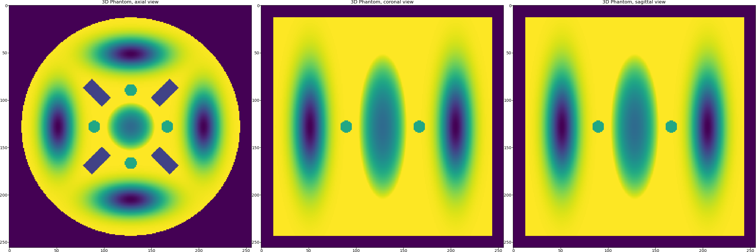
Once the phantom is generated we need to generate projection data, although the data in TomoPhantom is generated analytically and therefore it can be generated without the presence of the generated phantom.

# Parallel-beam projection geometry related parameters:
Horiz_det = int(np.sqrt(2) * N_size)  # detector column count (horizontal)
Vert_det = N_size  # detector row count (vertical) (no reason for it to be > N)
angles_num = int(0.5 * np.pi * N_size)
# angles number
angles = np.linspace(0.0, 179.9, angles_num, dtype="float32")  # in degrees
angles_rad = angles * (np.pi / 180.0) # in radians

projData3D_analyt = TomoP3D.ModelSino(
    model, N_size, Horiz_det, Vert_det, angles, path_library3D
)

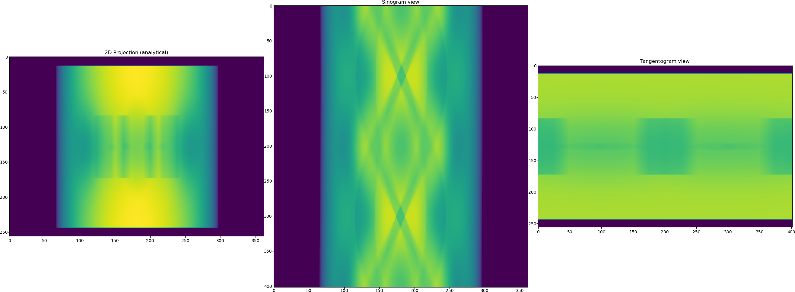
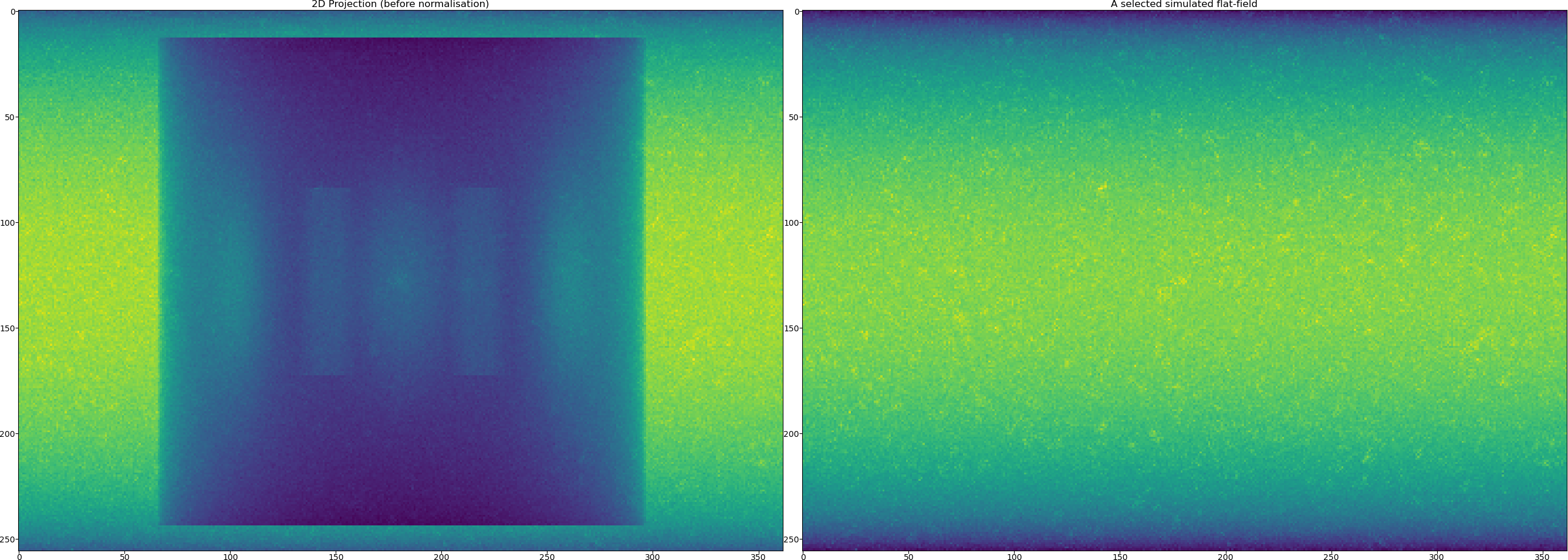
TomoPhantom offers a functionality to mimic flat fields that can be used later for normalisation. This normally leads to more realistic data generated. Note that the generated data has got the size of [256, 402, 362] with axes labels given as ["detY", "angles", "detX"]. We now generate flats and the data with the background from the ideal analytical data.

I0 = 15000 # Source intensity
flatsnum = 100  # the number of the flat fields simulated

[projData3D_noisy, flatsSIM, speckles] = synth_flats(
    projData3D_analyt, # ideal analytical data
    source_intensity=I0, # affects the amount of the Poisson noise added to data
    detectors_miscallibration=0.02, # A constant which perturbs some detectors positions
    arguments_Bessel=(1, 10, 10, 12), # control background low-freq variations
    specklesize=5, # Speckle size in pixel units for flats background simulation
    kbar=0.3, # Mean photon density (photons per pixel) for background simulation
    jitter_projections=0.0, # no jitter to projections
    sigmasmooth=3, # blurring the speckled backround
    flatsnum=flatsnum, # the number of flats
)

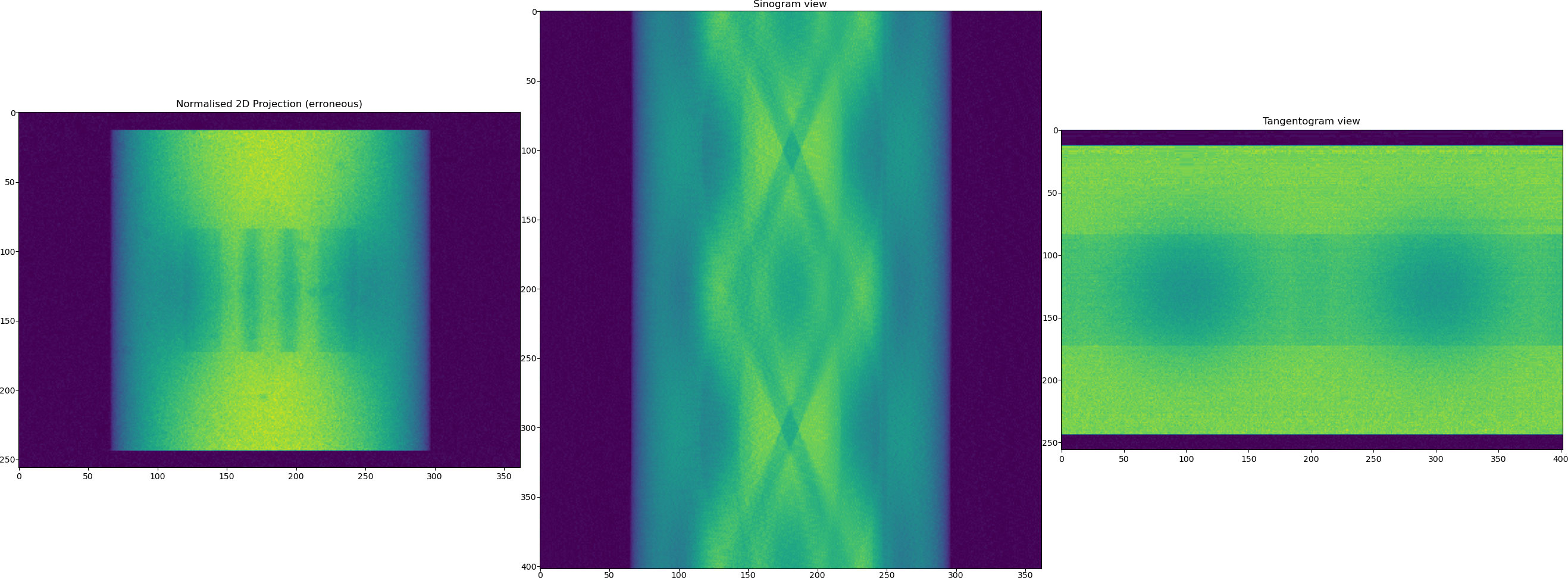
Projection data with background and the flat field

Now we normalise the data using the function from tomobar.supp.suppTools.normaliser. Note a visible stripe artefact in the generated sinogram after normalisation. This will result in a ring artefact in the reconstructed image.

projData3D_norm = normaliser(
projData3D_noisy, flatsSIM, darks=None, log="true", method="mean", axis=1
)

Now we are ready to perform reconstruction. Let us start with the direct reconstruction using Filtered Backprojection (FBP) method. Note the expected noisy reconstruction and the ring artefact.

from tomobar.methodsDIR import RecToolsDIR

RectoolsDIR = RecToolsDIR(
    DetectorsDimH=Horiz_det,  # DetectorsDimH # detector dimension (horizontal)
    DetectorsDimV=Vert_det,  # DetectorsDimV # detector dimension (vertical) for 3D case only
    CenterRotOffset=None,  # Center of Rotation (CoR) scalar (the data is perfectly centered here)
    AnglesVec=angles_rad,  # array of angles in radians
    ObjSize=N_size,  # a scalar to define reconstructed object dimensions
    device_projector="gpu",
)

data_axes_labels3D = ["detY", "angles", "detX"]
FBP_Rec = Rectools.FBP(projData3D_norm, data_axes_labels_order=data_axes_labels3D)

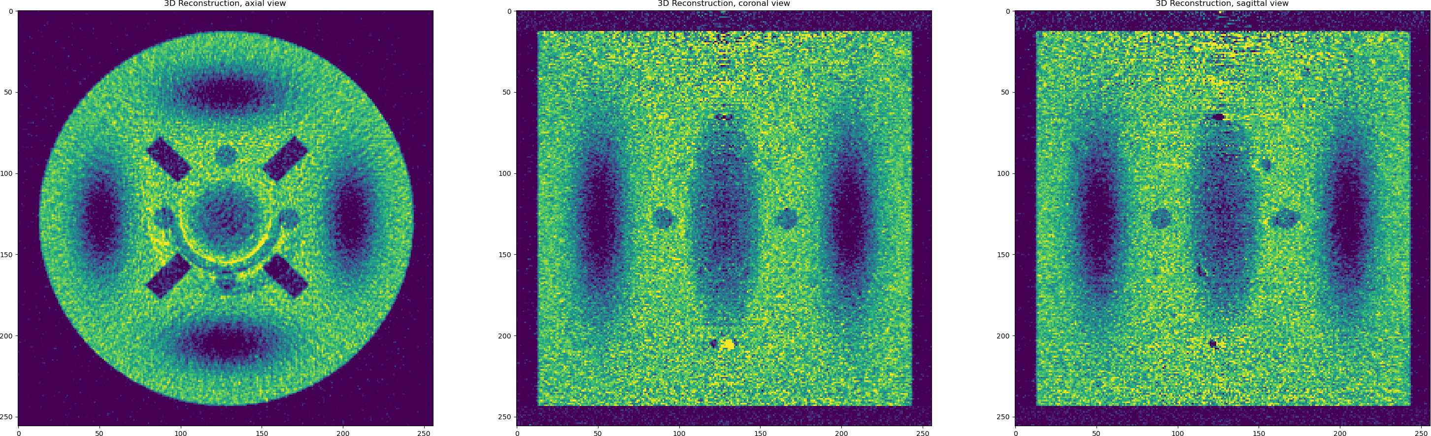
OK, so we have noisy data and artefacts and we achieved RMSE=0.2189 with FBP as a reconstruction error. Let us try to deal with each issue in the data one by one. First we apply iterative reconstruction with regularisation to minimise the noise.

Rectools = RecToolsIR(
    DetectorsDimH=Horiz_det,  # DetectorsDimH # detector dimension (horizontal)
    DetectorsDimV=Vert_det,  # DetectorsDimV # detector dimension (vertical) for 3D case only
    CenterRotOffset=None,  # Center of Rotation (CoR) scalar
    AnglesVec=angles_rad,  # array of angles in radians
    ObjSize=N_size,  # a scalar to define reconstructed object dimensions
    datafidelity="PWLS",  # data fidelity,
    device_projector="gpu",
)

_data_ = {
    "projection_norm_data": projData3D_norm,
    "projection_raw_data": projData3D_noisy / np.max(projData3D_noisy),
    "OS_number": 8, # the number of Ordered Subsets
    "data_axes_labels_order": ["detY", "angles", "detX"],
}  # data dictionary

lc = Rectools.powermethod(
    _data_
)  # calculate Lipschitz constant (run once to initialise)

# algorithm parameters
_algorithm_ = {"iterations": 15, "lipschitz_const": lc}

# regularisation dict
_regularisation_ = {
    "method": "PD_TV",
    "regul_param": 0.0000035, # Regularisation parameter for TV
    "iterations": 80,
    "device_regulariser": "gpu",
}

FISTA_TV = Rectools.FISTA(_data_, _algorithm_, _regularisation_)

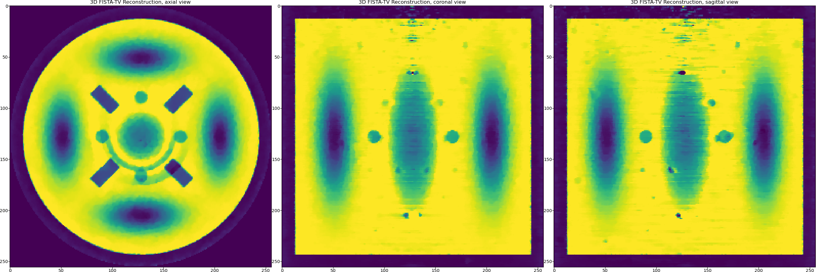
So using Total Variation with FISTA ordered-subsets we can achieve RMSE=0.048. We should also notice here that the TV penalty favours piecewise-constant solutions and we have smooth objects in our reconstructed data (Gaussians). So may be we should try a penalty that favours piecewise-smooth solution, a dual penalty like Total Generilised Variation or or even TV and Wavelet-based terms combined. Let us try the latter by modifying the regularisation dictionary and re-running the method.

# modifying regularisation dict
_regularisation_ = {
    "method": "PD_TV_WAVELETS",
    "regul_param": 0.0000035, # Regularisation parameter for TV
    "regul_param2": 0.000001,  # Regularisation parameter for wavelets
    "iterations": 80,
    "device_regulariser": "gpu",
}

FISTA_TV_WV = Rectools.FISTA(_data_, _algorithm_, _regularisation_)

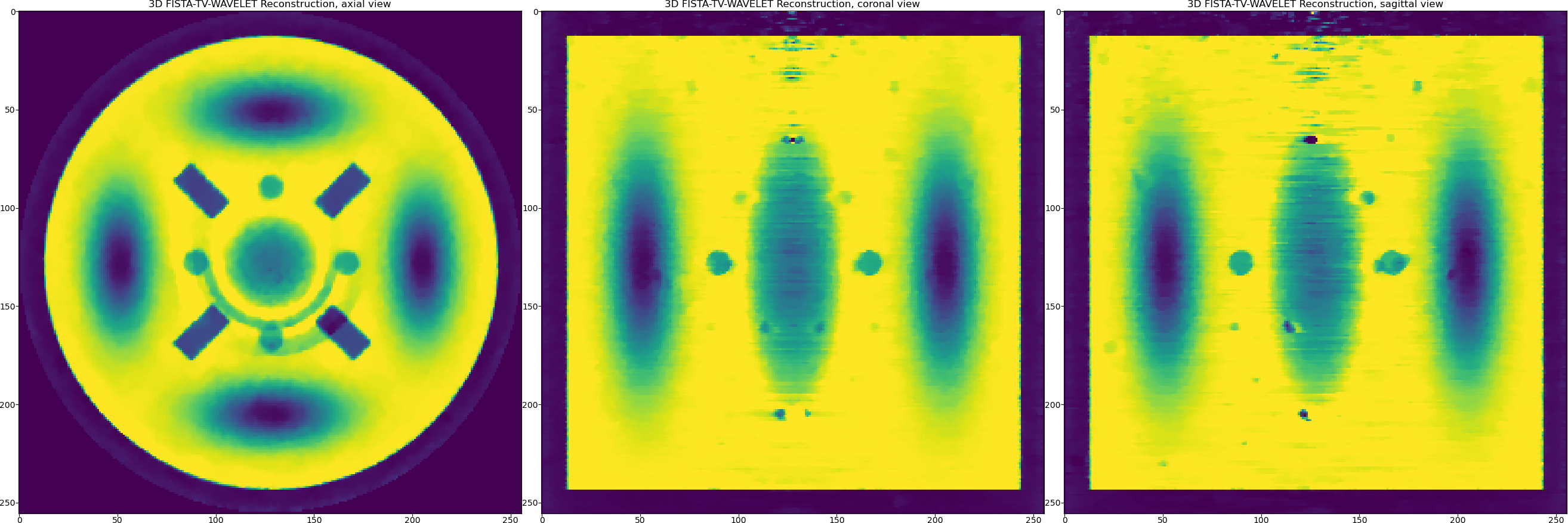
One can see that the reconstructed Gaussians look smoother while piecewise-constant objects are equally preserved. However, it is always a visual trade-off in terms of quality rather then relying on the minimisation of RMSE (it remains the same here). The structural similarity metrics might be a better choice.
Let us perform one last thing in attempt to remove ring artefacts in the reconstruction. We keep the same regulariser that produces the satisfying reconstruction but modify our data fidelity term. Please note that modifications of the data fidelity terms frequently lead to potentially unstable and non-convergent algorithms, so one needs to do that carefully. In ToMoBAR, there is at least a couple of data fidelity terms that can help with ring artefacts: Group-Huber [PM2015] penalty or Stripe-Weighted LS (SWLS) [HOA2017].

Rectools = RecToolsIR(
    DetectorsDimH=Horiz_det,  # Horizontal detector dimension
    DetectorsDimV=Vert_det,  # Vertical detector dimension (3D case)
    CenterRotOffset=None,  # Centre of Rotation scalar
    AnglesVec=angles_rad,  # A vector of projection angles in radians
    ObjSize=N_size,  # Reconstructed object dimensions (scalar)
    datafidelity="SWLS",  # Stripe Weighted LS  Data fidelity
    device_projector="gpu",
)

_data_ = {
    "projection_norm_data": projData3D_norm,
    "projection_raw_data": projData3D_noisy / np.max(projData3D_noisy),
    "beta_SWLS": 0.5, # SWLS related term
    "OS_number": 8, # the number of Ordered Subsets
    "data_axes_labels_order": ["detY", "angles", "detX"],
}  # data dictionary

lc = Rectools.powermethod(
    _data_
)  # calculate Lipschitz constant (run once to initialise)

_algorithm_ = {"iterations": 20, "lipschitz_const": lc}

# adding regularisation using the CCPi regularisation toolkit
_regularisation_ = {
    "method": "PD_TV_WAVELETS",
    "regul_param": 0.0000015, # Regularisation parameter for TV
    "regul_param2": 0.0000005,  # Regularisation parameter for wavelets
    "iterations": 80,
    "device_regulariser": "gpu",
}

FISTA_TV_WV_SWLS = Rectools.FISTA(_data_, _algorithm_, _regularisation_)

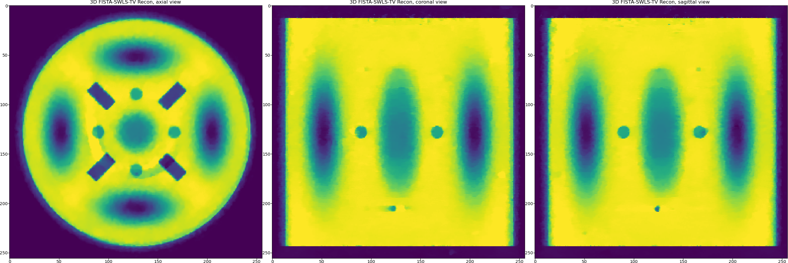
So we were able to minimise some ring artefacts which are the full ones (full angular stripe), but it is still problematic to minimise the partial ones with this model. However, with this example we would like to demonstrate the principle of the plug-and-play functionality of the ToMoBAR package.

One can also operate purely on CuPy arrays if Dependencies are satisfied for the CuPy package. For that one needs to use tomobar.methodsIR_CuPy class instead of tomobar.methodsIR. Note that the array of angles for the CuPy modules should be provided as a Numpy array.