Real data reconstruction

Warning

The results bellow presented using ToMoBAR version 2026.2.0.1. The class RecToolsIR is retired starting from version 2026.3.0.0 in favor of RecToolsIRCuPy. This demo will be updated soon.

Note

Installing HTTomolibGPU provides access to a wide range of GPU-accelerated processing tools, in addition to reconstruction wrappers that leverage ToMoBAR’s modules, see point 6 in Dependencies.

This tutorial demonstrates real data reconstruction using the ToMoBAR software. The dataset was acquired at the Diamond Light Source synchrotron facility (UK), on the i12 beamline. The sample is a magnesium alloy undergoing thermal cycling, during which dendritic growth occurs. See more details about the experiment in [GUO2018] and more on reconstruction using ToMoBAR in [KAZ2017].

This tutorial loosely follows Demo_RealData.py demo.

• We will extract a 2D sinogram out of 3D projection data and reconstruct it using the FBP method.

from tomobar.methodsDIR import RecToolsDIR

Rectools = RecToolsDIR(
    DetectorsDimH=detectorHoriz,  # Horizontal detector dimension
    DetectorsDimH_pad=0,  # Padding size of horizontal detector
    DetectorsDimV=None,  # Vertical detector dimension
    CenterRotOffset=None,  # Center of Rotation scalar
    AnglesVec=angles_rad,  # A vector of projection angles in radians
    ObjSize=N_size,  # Reconstructed object dimensions (scalar)
    device_projector="gpu",
)

FBPrec = Rectools.FBP(sinogram, data_axes_labels_order=["detX", "angles"])

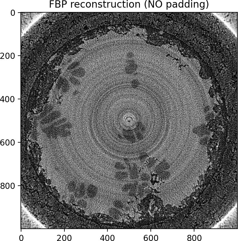
• In order to remove the circular artifact on the edges of the FBP reconstruction, one can edge-pad the horizontal detector.

from tomobar.methodsDIR import RecToolsDIR

Rectools = RecToolsDIR(
    DetectorsDimH=detectorHoriz,  # Horizontal detector dimension
    DetectorsDimH_pad=100,  # Padding size of horizontal detector
    DetectorsDimV=None,  # Vertical detector dimension
    CenterRotOffset=None,  # Center of Rotation scalar
    AnglesVec=angles_rad,  # A vector of projection angles in radians
    ObjSize=N_size,  # Reconstructed object dimensions (scalar)
    device_projector="gpu",
)

FBPrec = Rectools.FBP(sinogram, data_axes_labels_order=["detX", "angles"])

• Next we reconstruct using ordered-subsets FISTA with Total Variation regularisation.

from tomobar.methodsIR import RecToolsIR

Rectools = RecToolsIR(
    DetectorsDimH=detectorHoriz,  # Horizontal detector dimension
    DetectorsDimH_pad=0,  # Padding size of horizontal detector
    DetectorsDimV=None,  # Vertical detector dimension (3D case)
    CenterRotOffset=None,  # Center of Rotation scalar
    AnglesVec=angles_rad,  # A vector of projection angles in radians
    ObjSize=N_size,  # Reconstructed object dimensions (scalar)
    datafidelity="PWLS",  # Data fidelity term
    device_projector="gpu",
)

_data_ = {
    "projection_norm_data": sinogram,  # Normalised projection data
    "projection_raw_data": sinogram_raw,  # Raw projection data
    "OS_number": 6,  # The number of subsets
    "data_axes_labels_order": ["detX", "angles"],
}
lc = Rectools.powermethod(_data_)  # calculate Lipschitz constant

_algorithm_ = {"iterations": 25, "lipschitz_const": lc}

_regularisation_ = {
    "method": "PD_TV",  # Regularisation method
    "regul_param": 0.000002,  # Regularisation parameter
    "iterations": 60,  # The number of regularisation iterations
    "device_regulariser": "gpu",
}

RecFISTA = Rectools.FISTA(_data_, _algorithm_, _regularisation_)

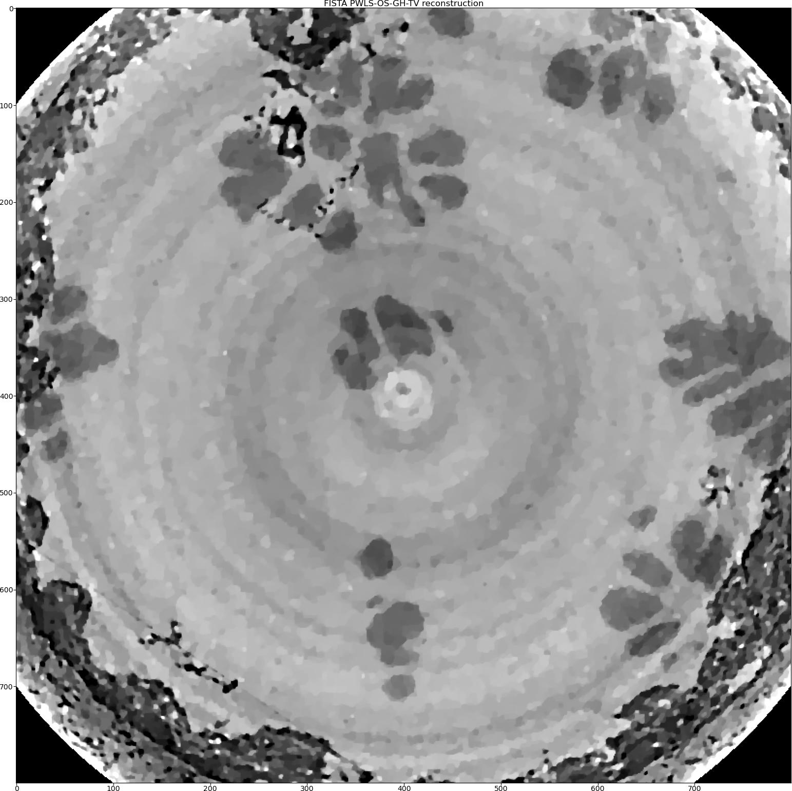
• Then we will add the Group-Huber data fidelity model [PM2015] to minimise the ring artefacts. We need to add new parameters to the _data_ dictionary.

_data_ = {
    "projection_norm_data": sinogram,  # Normalised projection data
    "projection_raw_data": sinogram_raw,  # Raw projection data
    "OS_number": 6,  # The number of subsets
    "data_axes_labels_order": ["detX", "angles"],
    "ringGH_lambda": 0.000015,
    "ringGH_accelerate": 6,
}

RecFISTA = Rectools.FISTA(_data_, _algorithm_, _regularisation_)

• We also can try the Stripe-Weighted Least Squares (SWLS) data model [HOA2017]. As we change the data fidelity, we need to re-initialise the geometry object.

Rectools = RecToolsIR(
    DetectorsDimH=detectorHoriz,  # Horizontal detector dimension
    DetectorsDimH_pad=0,  # Padding size of horizontal detector
    DetectorsDimV=None,  # Vertical detector dimension (3D case)
    CenterRotOffset=None,  # Center of Rotation scalar
    AnglesVec=angles_rad,  # A vector of projection angles in radians
    ObjSize=N_size,  # Reconstructed object dimensions (scalar)
    datafidelity="SWLS",  # Data fidelity term
    device_projector="gpu",
)

_data_ = {
    "projection_norm_data": sinogram,  # Normalised projection data
    "projection_raw_data": sinogram_raw,  # Raw projection data
    "OS_number": 6,  # The number of subsets
    "beta_SWLS": 0.2,  #  parameter for the SWLS model
    "data_axes_labels_order": ["detX", "angles"],
}

RecFISTA = Rectools.FISTA(_data_, _algorithm_, _regularisation_)

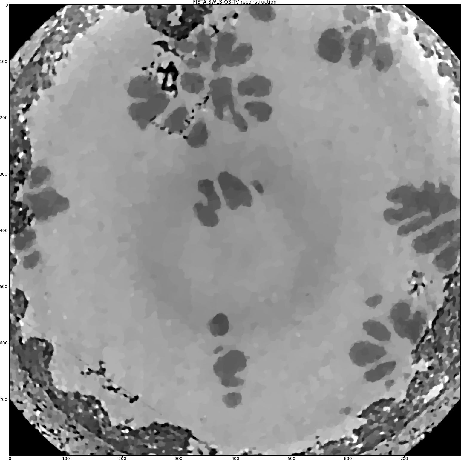
As one can see that visually the SWLS model produced the best reconstruction here. This model is indeed works very well when the stripes (rings) are full and not partial.